Simple Linear Regression with Minitab

What is Simple Linear Regression?

Simple linear regression is a statistical technique to fit a straight line through the data points. It models the quantitative relationship between two variables. It is simple because only one predictor variable is involved. It describes how one variable changes according to the change of another variable. Both variables need to be continuous; there are other types of regression to model discrete data.

Simple Linear Regression Equation

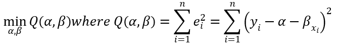
The simple linear regression analysis fits the data to a regression equation in the form

Where:

[unordered_list style=”star”]

• Y is the dependent variable (the response) and X is the single independent variable (the predictor)
• α is the slope describing the steepness of the fitting line. β is the intercept indicating the Y value when X is equal to 0
• e stands for error (residual). It is the difference between the actual Y and the fitted Y (i.e. the vertical difference between the data point and the fitting line).

Ordinary Least Squares

The ordinary least squares is a statistical method used in linear regression analysis to find the best fitting line for the data points. It estimates the unknown parameters of the regression equation by minimizing the sum of squared residuals (i.e. the vertical difference between the data point and the fitting line).

In mathematical language, we look for α and β that satisfy the following criteria:

The actual value of the dependent variable:

Where: i = 1, 2 . . . n.

The fitted value of the dependent variable:

Where: i = 1, 2 . . . n.

By using calculus, it can be shown the sum of squared error is minimal when

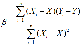
and

ANOVA in Simple Linear Regression

[unordered_list style=”star”]

• X: the independent variable that we use to predict;
• Y: the dependent variable that we want to predict.

[/unordered_list]

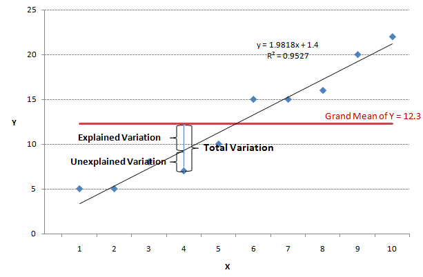
The variance in simple linear regression can be expressed as a relationship between the actual value, the fitted value, and the grand mean—all in terms of Y.

[unordered_list style=”star”]

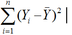
• Total Variation = Total Sums of Squares =  
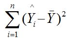
• Explained Variation = Regression Sums of Squares = 
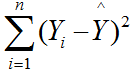
• Unexplained Variation = Error Sums of Squares = 

[/unordered_list]

Regression follows the same methodology as ANOVA and the hypothesis tests behind it use the same assumptions.

Variation Components

i.e. Total Sums of Squares = Regression Sums of Squares + Error Sums of Squares

Degrees of Freedom Components

i.e. n – 1 = (k – 1) + (n – k), where n is the number of data points, k is the number of predictors

Whether the overall model is statistically significant can be tested by using F-test of ANOVA.

[unordered_list style=”star”]

• H₀: The model is not statistically significant.
• H_a: The model is statistically significant.

[/unordered_list]

Test Statistic

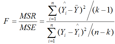
Critical Statistic

Is represented by F value in F table with (k – 1) degrees of freedom in the numerator and (n – k) degrees of freedom in the denominator.

[unordered_list style=”star”]

• If F ≤ F_critical (calculated F is less than or equal to the critical F), we fail to reject the null. There is no statistically significant relationship between X and Y.
• If F > F_critical, we reject the null. There is a statistically significant relationship between X and Y.

[/unordered_list]

Coefficient of Determination

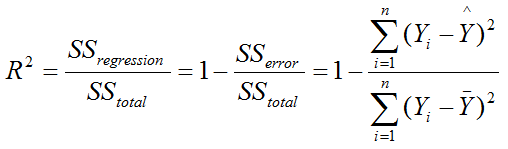
R-squared or R² (also called coefficient of determination) measures the proportion of variability in the data that can be explained by the model.

[unordered_list style=”star”]

• R² ranges from 0 to 1. The higher R² is, the better the model can fit the actual data.
• R² can be calculated with the formula:

[/unordered_list]

Use Minitab to Run a Simple Linear Regression

Case study: We want to see whether the score on exam one has any statistically significant relationship with the score on the final exam. If yes, how much impact does exam one have on the final exam?
Data File: “Simple Linear Regression” tab in “Sample Data.xlsx”

Step 1: Determine the dependent and independent variables. Both should be continuous variables.

[unordered_list style=”star”]

• Y (dependent variable) is the score of final exam.
• X (independent variable) is the score of exam one.

[/unordered_list]

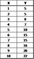
Step 2: Create a scatter plot to visualize whether there seems to be a linear relationship between X and Y.

1. Click Graph → Scatterplot.
2. A new window named “Scatterplots” pops up.
3. Click “OK.”
4. A new window named “Scatterplot– Simple” pops up.
5. Select “FINAL” as “Y variables” and “EXAM1” as “X variables.”
   
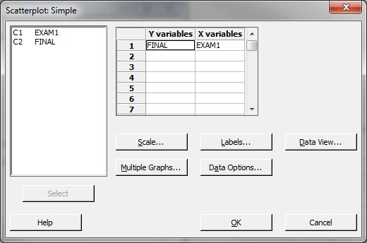
6. Click “OK.”
7. A scatter plot is generated in a new window.
   

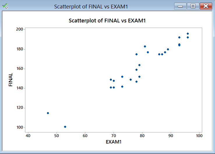
Based on the scatter plot, the relationship between exam one and final seems linear. The higher the score on exam one, the higher the score on the final. It appears you could “fit” a line through these data points.

Step 3: Run the simple linear regression analysis.

1. Click Stat → Regression → Regression → Fit Regression Model.
2. A new window named “Regression” pops up.
3. Select “FINAL” as “Response” and “EXAM1” as “Continuous Predictors.”
   
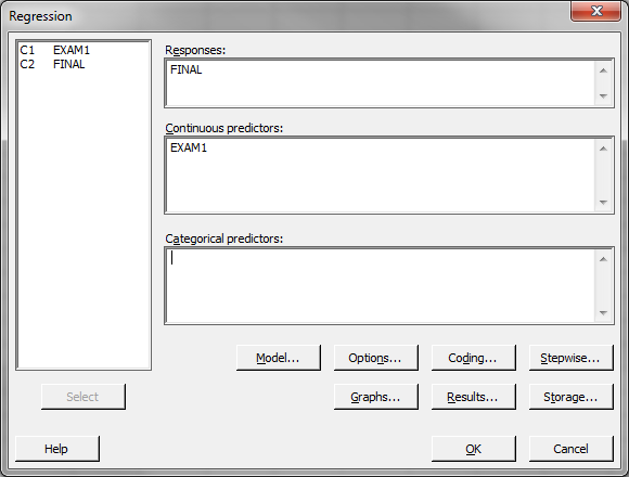
4. Click the “Storage” button.
5. Check the box of “Residuals” so that the residuals can be saved automatically in the last column of the data table.
   
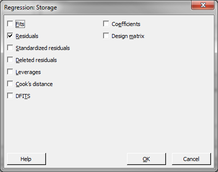
6. Click “OK.”
7. The regression analysis results appear in the new window.
   

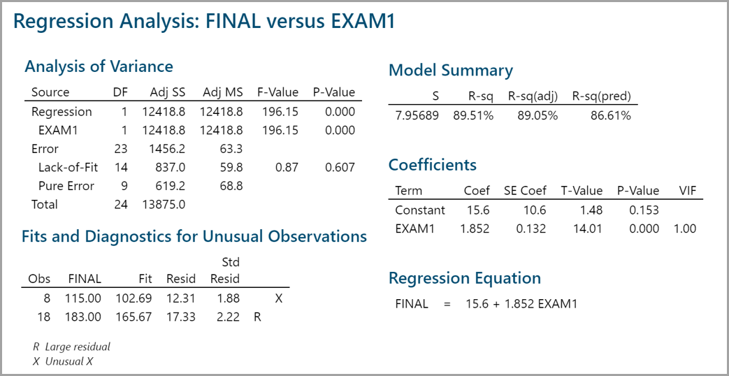
Step 4: Check whether the model is statistically significant. If not significant, we will need to re-examine the predictor or look for new predictors before continuing. R² measures the percentage of variation in the data set that can be explained by the model. 89.5% of the variability in the data can be accounted for by this linear regression model. “Analysis of Variance” section provides an ANOVA table covering degrees of freedom, sum of squares, and mean square information for total, regression and error. The p-value of the F-test is lower than the α level (0.05), indicating that the model is statistically significant.

The p-value is 0.0001; therefore, we reject the null and claim the model is statistically significant. The R square value says that 89.5% of the variability can be explained by this model.

Step 5: Understand regression equation

The estimates of slope and intercept are shown in “Parameter Estimate” section. In this example, Y = 15.6 + 1.85 × X, where X is the score on Exam 1 and Y is the final exam score. One unit increase in the score of Exam1 would increase the final score by 1.85.

Interpreting the Results

Let us say you are the professor and you want to use this prediction equation to estimate what two of your students might get on their final exam.

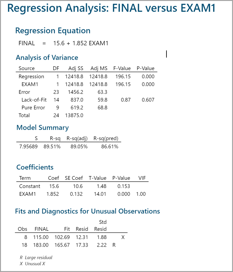
Rsquare Adj = 89.0%

[unordered_list style=”star”]

• 89% of the variation in FINAL can be explained by EXAM1

[/unordered_list]

P-value of the F-test = 0.000

[unordered_list style=”star”]

• We have a statistically significant model

[/unordered_list]

Prediction Equation: 15.6 + 1.85 × EXAM1

[unordered_list style=”star”]

• 6 is the Y intercept, all equations will start with 15.6
• 85 is the EXAM1 Coefficient: multiply it by EXAM1 score

[/unordered_list]

Because the model is significant, and it explains 89% of the variability, we can use the model to predict final exam scores based on the results of Exam1.

Let us assume the following:

[unordered_list style=”star”]

• Student “A” exam 1 results were: 79
• Student “B” exam 1 results were: 94

[/unordered_list]

Remember our prediction equation 15.6 + 1.85 × Exam1?

Now apply the equation to each student:

Student “A” Estimate: 15.6 + (1.85 × 79) = 161.8

Student “B” Estimate: 15.6 + (1.85 × 94) = 189.5

Model summary: By simply replacing exam 1 scores into the equation we can predict their final exam scores. But the key thing about the model is whether or not it is useful. In this case, the professor can use the results to Figure out where to spend his time helping students.