Kruskal Wallis Test with Minitab

Kruskal Wallis One-Way Analysis of Variance

The Kruskal Wallis one-way analysis of variance is a statistical hypothesis test to compare the medians among more than two groups.

[unordered_list style=”star”]

• Null Hypothesis (H0): η1 = η2 = … = ηk
• Alternative Hypothesis (Ha): at least one of the medians is different from others
  Where:
• ηi is the median of population i
• k is the number of groups of our interest

[/unordered_list]

It is an extension of Mann–Whitney test. While the Mann–Whitney test allows us to compare the samples of two populations, the Kruskal–Wallis test allows us to compare the samples of more than two populations.
One key difference between this test and the Mann–Whitney test is the robustness of the test when the populations are not identically shaped. If this is the case, there is a different test, called Mood’s median, which is more appropriate.

Kruskal Wallis One-Way Analysis of Variance: Assumptions

[unordered_list style=”star”]

• The sample data drawn from the populations of interest are unbiased and representative.
• The data of k populations are continuous or ordinal when the spacing between adjacent values is not constant.
• The k populations are independent to each other.
• The Kruskal–Wallis test is robust for the non-normally distributed population.

[/unordered_list]

How Kruskal Wallis One-Way ANOVA Works

The Kruskal–Wallis test works very similarly to the Mann–Whitney Test.
Step 1: Group the k samples from k populations (sample i is from population i) into one single data set and then sort the data in ascending order ranked from 1 to N, where N is the total number of observations across k groups.
Step 2: Add up the ranks for all the observations from sample i and call it ri, where i can be any integer between 1 and k.

Step 3: Calculate the test statistic
Where:

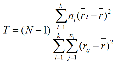
[unordered_list style=”star”]

• k is the number of groups
• ni is the sample size of sample i
• N is the total number of all the observations across k groups
• rij is the rank (among all the observations) of observation j from group i

[/unordered_list]

Step 4: Make a decision of whether to reject the null hypothesis.

[unordered_list style=”star”]

• Null Hypothesis (H0): η1 = η2 =…= ηk
• Alternative Hypothesis (Ha): at least one of the medians is different from others

[/unordered_list]

The test statistic follows chi-square distribution when the null hypothesis is true. If T is greater than(the critical chi-square statistic), we reject the null and claim there is at least one median statistically different from other medians. If T is smaller than, we fail to reject the null and claim the medians of k groups are equal.

Use Minitab to Run a Kruskal–Wallis One-Way ANOVA

Case study: We are interested in comparing customer satisfaction among three types of customers using a nonparametric (i.e. distribution-free) hypothesis test: Kruskal–Wallis one-way ANOVA.
Data File: “Kruskal–Wallis” tab in “Sample Data.xlsx”

[unordered_list style=”star”]

• Null Hypothesis (H₀): η₁ = η₂ = η₃
• Alternative Hypothesis(H_a): at least one of the customer types has different overall satisfaction levels from the others

[/unordered_list]

Steps to run a Kruskal–Wallis One-Way ANOVA in Minitab

1. Click Stat → Nonparametrics → Kruskal–Wallis.
2. A new window named “Kruskal–Wallis” pops up.
3. Select “Overall Satisfaction” as the “Response.”
4. Select “Customer Type” as the “Factor.”
   
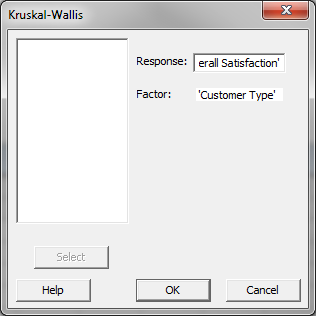
5. Click “OK.”
6. The Kruskal–Wallis test results appear in the session window.
   

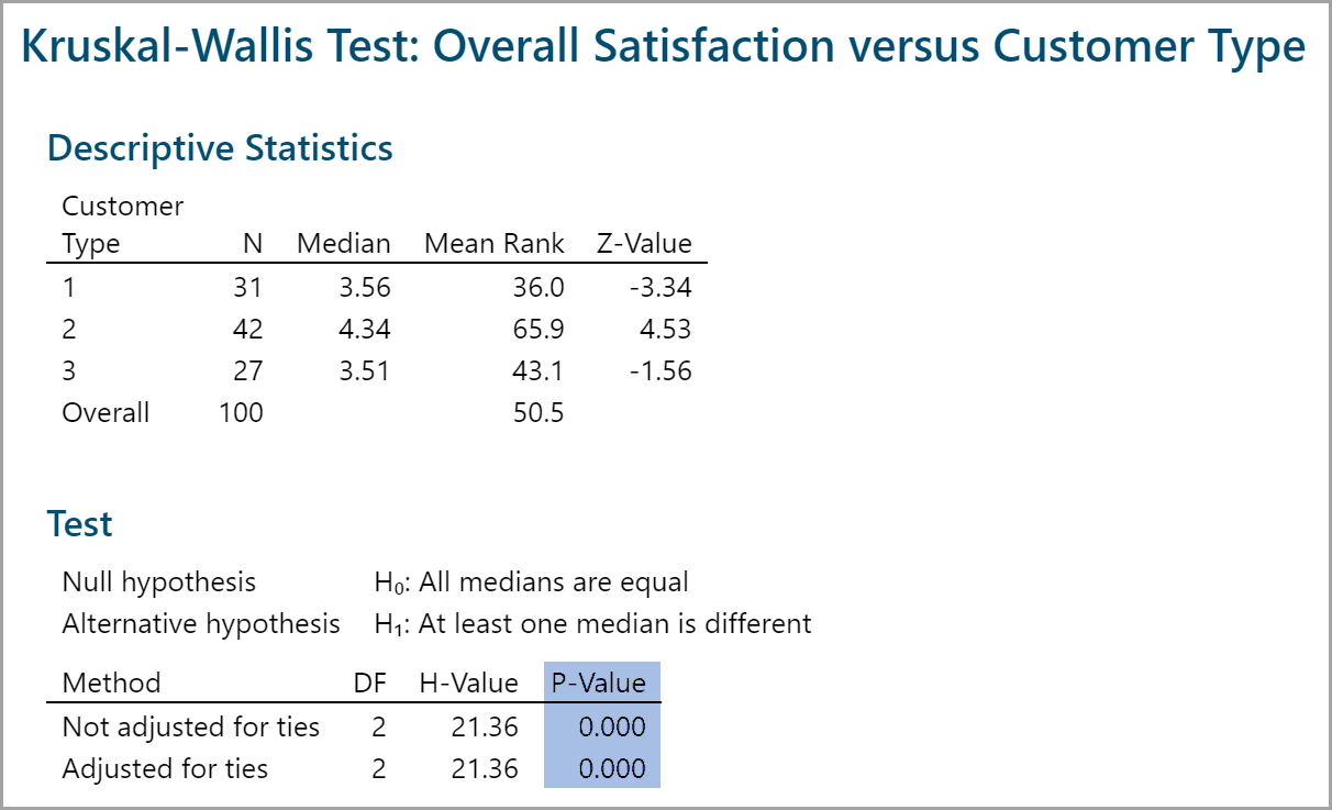
Model summary: The p-value of the test is lower than alpha level (0.05), and we reject the null hypothesis and conclude that at least the overall satisfaction median of one customer type is statistically different from the others.